
Frequency Response of an electric or electronics circuit allows us to see exactly how the output gain (known as the magnitude response) and the phase (known as the phase response) changes at a particular single frequency, or over a whole range of different frequencies from 0Hz, (d.c.) to many thousands of mega‐hertz, (MHz) depending upon the design characteristics of the circuit.
Generally, the frequency response analysis of a circuit or system is shown by plotting its gain, that is the size of its output signal to its input signal, Output/Input against a frequency scale over which the circuit or system is expected to operate. Then by knowing the circuits gain, (or loss) at each frequency point helps us to understand how well (or badly) the circuit can distinguish between signals of different frequencies.
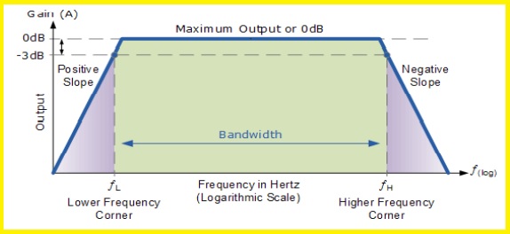
The frequency response of a given frequency dependent circuit can be displayed as a graphical sketch of magnitude (gain) against frequency (ƒ). The horizontal frequency axis is usually plotted on a logarithmic scale while the vertical axis representing the voltage output or gain, is usually drawn as a linear scale in decimal divisions. Since a systems gain can be both positive or negative, the y‐axis can therefore have both positive and negative values
Frequency Response Curve
Audio
Amplifier
An amplifier designed for audio frequency amplification will amplify signals with a frequency of less than about 20kHz but will not amplify signals having higher frequencies. An amplifier designed for radio frequencies will amplify a band of frequencies above about 100kHz but will not amplify the lower frequency audio signals. In each case the amplifier has a particular frequency response, being a band of frequencies where it provides adequate amplification, and excluding frequencies above and below this band, where the amplification is less than adequate.

Fig. 1.1.1b Response curve for a RF amplifier tuned to 774kHz
To show how the gain of an amplifier varies with frequency, a graph, showing the frequency response of the amplifier is used. Fig. 1.1.1a shows the typical frequency response curve of an audio amplifier, and Fig. 1.1.1b, that of a RF amplifier. In such graphs, it is common that very large values may be encountered for both gain and frequency. For this reason it is usual for both the frequency and gain axes of the graph to use logarithmic scales. It can be seen from Fig. 1.1.1a that scales on the (horizontal) x‐axis do not increase in a linear manner; each equal division represents a tenfold increase in the frequency plotted. This ensures that a very wide range of frequency can be plotted on a single graph. The (vertical) y‐axis uses linear divisions but logarithmic units (deciBels dB). The curve of the graph shows how gain, measured in deciBels, varies with frequency.
Comparing Figs. 1.1.1a and b drawn in this manner, shows how each type of amplifier (audio, RF etc) has its own characteristic shape of frequency response curve. An amplifier which has a very narrow, sharply peaked response curve is said to be very "selective". This is typical of an RF amplifier and is precisely what is needed in an amplifier designed for the tuning stages of a radio where only one radio carrier wave among many hundred others, crowded along the medium wave band for example, must be selected.
Intermediate frequency
In communications and electronic engineering, an intermediate frequency (IF) is a frequency to which a carrier frequency is shifted as an intermediate step in transmission or reception.[1] The intermediate frequency is created by mixing the carrier signal with a local oscillator signal in a process called heterodyning, resulting in a signal at the difference or beat frequency. Intermediate frequencies are used in superheterodyne radio receivers, in which an incoming signal is shifted to an IF for amplification before final detection is done
Commonly used intermediate frequencies
- 110 kHz was used in Long wave broadcast receivers.[1]
- Analogue television receivers using system M: 41.25 MHz (audio) and 45.75 MHz (video). Note, the channel is flipped over in the conversion process in an intercarrier system, so the audio IF frequency is lower than the video IF frequency. Also, there is no audio local oscillator; the injected video carrier serves that purpose.
- Analogue television receivers using system B and similar systems: 33.4 MHz for aural and 38.9 MHz for visual signal. (The discussion about the frequency conversion is the same as in system M).
- FM radio receivers: 262 kHz, 455 kHz, 1.6 MHz, 5.5 MHz, 10.7 MHz, 10.8 MHz, 11.2 MHz, 11.7 MHz, 11.8 MHz, 21.4 MHz, 75 MHz and 98 MHz
- AM radio receivers: 450 kHz, 455 kHz, 460 kHz, 465 kHz, 467 kHz, 470 kHz, 475 kHz, 480 kHz.[7]
- Satellite uplink‐downlink equipment: 70 MHz, 950‐1450 MHz (L‐Band) Downlink first IF.
- Terrestrial microwave equipment: 250 MHz, 70 MHz or 75 MHz
- Radar: 30 MHz
- RF Test Equipment: 310.7 MHz, 160 MHz, 21.4 MHz
Video amplifier
A low‐pass amplifier having a bandwidth in the range from 2 to 100 MHz. Typical applications are in television receivers, cathode‐ray‐tube computer terminals, and pulse amplifiers. The function of a video amplifier is to amplify a signal containing high‐frequency components without introducing distortion.
Modern video amplifiers use specially designed integrated circuits. With one chip and an external resistor to control the voltage gain, it is possible to make a video amplifier with a bandwidth between 50 and 100 MHz having voltage gains ranging from 20 to 500. See Amplifier, Integrated circuits.
A wideband amplifier has a precise amplification factor over a wide frequency range, and is often used to boost signals for relay in communications systems. A narrowband amp amplifies a specific narrow range of frequencies, to the exclusion of other frequencies.
Bandwidth
Bandwidth is the difference between the upper and lower frequencies in a continuous set of frequencies. It is typically measured in hertz, and may sometimes refer to passband bandwidth, sometimes to baseband bandwidth, depending on context. Passband bandwidth is the difference between the upper and lower cutoff frequencies of, for example, a bandpass filter, a communication channel, or a signal spectrum. In the case of a low‐pass filter or baseband signal, the bandwidth is equal to its upper cutoff frequency.
Signal to Noise Ratio, SNR
The noise performance and hence the signal to noise ratio is a key parameter for any radio receiver. The signal to noise ratio, or SNR as it is often termed is a measure of the sensitivity performance of a receiver. This is of prime importance in all applications from simple broadcast receivers to those used in cellular or wireless communications as well as in fixed or mobile radio communications, two way radio communications systems, satellite radio and more.
There are a number of ways in which the noise performance, and hence the sensitivity of a radio receiver can be measured. The most obvious method is to compare the signal and noise levels for a known signal level, i.e. the signal to noise (S/N) ratio or SNR. Obviously the greater the difference between the signal and the unwanted noise, i.e. the greater the S/N ratio or SNR, the better the radio receiver sensitivity performance. As with any sensitivity measurement, the performance of the overall radio receiver is determined by the performance of the front end RF amplifier stage. Any noise introduced by the first RF amplifier will be added to the signal and amplified by subsequent amplifiers in the receiver. As the noise introduced by the first RF amplifier will be amplified the most, this RF amplifier becomes the most critical in terms of radio receiver sensitivity performance. Thus the first amplifier of any radio receiver should be a low noise amplifier.
Concept of signal to noise ratio SNR
Although there are many ways of measuring the sensitivity performance of a radio receiver, the S/N ratio or SNR is one of the most straightforward and it is used in a variety of applications. However it has a number of limitations, and although it is widely used, other methods including noise figure are often used as well. Nevertheless the S/N ratio or SNR is an important specification, and is widely used as a measure of receiver sensitivity

The difference is normally shown as a ratio between the signal and the noise (S/N) and it is normally expressed in decibels. As the signal input level obviously has an effect on this ratio, the input signal level must be given. This is usually expressed in microvolts. Typically a certain input level required to give a 10 dB signal to noise ratio is specified.
Signal to noise ratio formula
The signal to noise ratio is the ratio between the wanted signal and the unwanted background noise.

It is more usual to see a signal to noise ratio expressed in a logarithmic basis using decibels:

If all levels are expressed in decibels, then the formula can be simplified to:
The power levels may be expressed in levels such as dBm (decibels relative to a milliwatt, or to some other standard by which the levels can be compared.
Effect of bandwidth on SNR
A number of other factors apart from the basic performance of the set can affect the signal to noise ratio, SNR specification. The first is the actual bandwidth of the receiver. As the noise spreads out over all frequencies it is found that the wider the bandwidth of the receiver, the greater the level of the noise. Accordingly the receiver bandwidth needs to be stated.
Additionally it is found that when using AM the level of modulation has an effect. The greater the level of modulation, the higher the audio output from the receiver. When measuring the noise performance the audio output from the receiver is measured and accordingly the modulation level of the AM has an effect. Usually a modulation level of 30% is chosen for this measurement. gain‐bandwidth product
- A figure of merit for amplifiers, especially operational amplifiers. It may be expressed in various manners, such as the product of the gain of an amplifier and its bandwidth. Its abbreviation is GBP
- The gain–bandwidth product (designated as GBWP, GBW, GBP or GB) for an amplifier is the product of the amplifier's bandwidth and the gain at which the bandwidth is measured
For transistors, the current‐gain–bandwidth product is known as the fT or transition frequency.It is calculated from the low‐frequency (a few kilohertz) current gain under specified test conditions, and the cutoff frequency at which the current gain drops by 3 decibels (70% amplitude); the product of these two values can be thought of as the frequency at which the current gain would drop to 1, and the transistor current gain between the cutoff and transition frequency can be estimated by dividing fT by the frequency. Usually, transistors must be applied at frequencies well below fT to be useful as amplifiers and oscillators.[5] In a bipolar junction transistor, frequency response declines owing to the internal capacitance of the junctions. The transition frequency varies with collector current, reaching a maximum for some value and declining for greater or lesser collector current


0 Comments
If you have any doubts, please let me know